原始論文為〈Zum elektrischen Widerstandsgesetz bei tiefen Temperaturen〉,因為 Google 翻成英文後的排版很亂,所以想說就把它打上來,也許比較看得懂,結果其實我也沒看很懂(暈)。
A solution method is given which allows to determine the stationary velocity distribution of the conduction electrons under the influence of an external electric field for low temperatures. A law is obtained for electrical resistance.
Some time ago we examined the interaction processes of the conduction electrons with the crystal lattice and showed that its elastic oscillations cause not only changes in momentum but also changes in energy for the electrons. The question of a distribution function that is stationary under the influence of an external electric field and the lattice vibrations, and consequently of the resistance, then leads to a linear integral equation, while in the theories of Lorentz and Houston one finds where the energy changes of the electrons are neglected, only has to solve an ordinary linear equation for the distribution function **.
A solution could easily be found far above the characteristic temperature $\Theta$ of the metal, since there the energy of the lattice vibrations changes relatively little as a result of the interaction with the electrons. On the other hand, at that time we did not succeed in finding a solution for $T\ll\Theta$, and the assumption that the low temperatures cause substantial exchange of energy, together with Pauli’s exclusion principle, the disappearance of resistance with temperature, could not find any rigorous quantitative justification. This should be done here.
In discussing the integral equation (82), 1. c., for $T\ll\Theta$, we mistakenly believed that the terms with $\left(\frac{T}{\Theta}\right)^2$ on the left-hand side to be allowed to neglect (cf. p.598, 1. c.). But this must not happen, because otherwise the homogeneous equation that one obtains if one sets the right-hand side in (82) to zero, has the solution $c(\varepsilon)=const.$ and therefore, as one can easily see, the inhomogeneous equation (82) would have no finite solution at all. Therefore, one must not, as in 1. c., derive the temperature dependence of the function $c(\varepsilon)$ sought from the right-hand side of (82) and, as we shall see, a $T^3$ law follows from our model instead of a $T^5$ law for the resistance.
In order to get a solution valid for low temperatures, we just use the fact mentioned above, that then the homogeneous equation has an approximate solution. Its physical meaning becomes clear by going back to equation (77), 1. c., used to determine the steady-state distribution function
$$f=f_0(E)+\xi\chi(E)\label{1}\tag{1}$$
serves
$$\begin{align*}c_1\left(\frac{T}{\Theta}\right)^3\int_{x=0}^{\Theta/T}\int_{\phi=0}^{2\pi}\frac{x^2dxd\phi}{e^x-1}\left\{\xi\chi(E)\frac{f_0(E+kTx)e^x+f_0(E-kTx)}{f_0(E)}\right.&&\\[5pt]-\xi^\prime\left.\left[\chi(E+kTx)\frac{f_0(E)}{f_0(E+kTx)}+\chi(E-kTx)\frac{f_0(E)e^x}{f_0(E-kTx)}\right]\right\}&&\\[5pt]=-c_2 F\xi\frac{\partial f_0}{\partial \rho}.&&\label{2}\tag{2}\end{align*}$$
On the left is the number of electrons leaving a state with energy $E$ as a result of the interaction with the lattice per unit time, and on the left is the number of electrons entering as a result of the field $F$ in the $x$-direction; both must be equal for stationarity to exist, $\xi$ and $\rho$ are proportional to the $x$ component or the absolute value of the velocity, $f_0$ is the Fermi distribution function, $c_1$ and $c_2$ are constants. For low temperatures, not only is the frequency of the transitions possible for the electrons generally smaller, but it will only be noticeable for transitions in which the momentum of the electrons changes little, since the long elastic waves, which are then mainly only involved, can only give rise to such transitions according to the interference condition (60a), 1. c. However, if one neglects the change in the $x$-component of the electron momentum entirely, by putting $\xi$ in (2) instead of $\xi^\prime$, or by omitting the $\left(\frac{T}{\Theta}\right)^2$ terms in (82), which means the same thing, then, of course, no stationary distribution can occur under the influence of an accelerating field.
We therefore write $\xi^\prime=\xi-X$ and bring the terms with $X$ to the right-hand side:
$$\begin{align*}c_1\left(\frac{T}{\Theta}\right)^3\int_{x=0}^{\Theta/T}\int_{\phi=0}^{2\pi}\frac{x^2dxd\phi}{e^x-1}\xi\left\{\chi(E)\frac{f_0(E+kTx)e^x+f_0(E-kTx)}{f_0(E)}\right.&&\\[5pt]\left.-\chi(E+kTx)\frac{f_0(E)}{f_0(E+kTx)}-\chi(E-kTx)\frac{f_0(E)e^x}{f_0(E-kTx)}\right\}&&\\[5pt]=-c_2F\chi\frac{\partial f_0}{\partial \rho}-c_1\left(\frac{T}{\Theta}\right)^3\int_{x=0}^{\Theta/T}\int_{\phi=0}^{2\pi}\frac{x^2dxd\phi}{e^x-1}X\left\{\chi(E+kTx)\frac{f_0(E)}{f_0(E+kTx)}\right.&&\\[5pt]\left.+\chi(E-kTx)\frac{f_0(E)e^x}{f_0(E-kTx)}\right\}.\label{3}\tag{3}\end{align*}$$
Setting the right-hand side of (3) to zero, the solution of the homogeneous equation is $\chi_1(E)=\alpha\frac{df_0}{dE}$, where $\alpha$ is an arbitrary constant, and this means that in the absence of an external perturbation and as long as one only considers processes where does not change not only $f_0(E)$ but also for small values of $\alpha$
$$f=f_0(E)+\xi\chi_1(E)=f_0(E)+\alpha\xi\frac{df_0}{dE}\approx f_0(E+\alpha\xi)$$
represents a stationary distribution, since this only requires an additional constant $\xi$ in the energy for the states with the same, between which transitions take place.
For approximate solution of (3), we now set
$$\begin{align*}\chi=\chi_1+\chi_2=\alpha\frac{df_0}{dE}+\chi_2\label{4}\tag{4}\end{align*}$$
and show that the constant $\alpha$ can be determined such that $\chi_2\ll\chi_1$, so that in the first-order approximation on the right-hand side of (3), $\chi_2$ can be neglected. One then gets like this
$$\begin{align*}c_1\left(\frac{T}{\Theta}\right)^3\int_{x=0}^{\Theta/T}\int_{\phi=0}^{2\pi}\frac{x^2dxd\phi}{e^x-1}\chi\left\{\chi_2(E)\frac{f_0(E+kTx)e^x+f_0(E-kTx)}{f_0(E)}\right.&&\\[5pt]\left.-\chi_2(E+kTx)\frac{f_0(E)}{f_0(E+kTx)}-\chi_2(E-kTx)\frac{f_0(E)e^x}{f_0(E-kTx)}\right\}&&\\[5pt]=-c_2F\xi\frac{\partial f_0}{\partial \rho}-c_1\left(\frac{T}{\Theta}\right)^3\int_{x=0}^{\Theta/T}\int_{\phi=0}^{2\pi}\frac{x^2dxd\phi}{e^x-1}X\left\{\chi_1(E+kTx)\frac{f_0(E)}{f_0(E+kTx)}\right.&&\\[5pt]\left.+\chi_1(E-kTx)\frac{f_0(E)e^x}{f_0(E-kTx)}\right\}.\label{5}\tag{5}\end{align*}$$
In order for (5) to have a finite solution $\chi_2$, it is known that the solution of the transposed homogeneous equation must be orthogonal to the right-hand side. It is easy to verify that this solvability condition is equivalent to the one immediately evident from (5) that the right-hand side integrated over $E$ from $-\infty$ to $+\infty$ much vanish since this condition is satisfied for the left-hand side; it simply expresses there that under the influence of transitions in which $\xi$ does not change, the number of electrons with fixed $\xi$ is constant in time. That the lower bound for $E$ can be taken as $-\infty$ instead of $0$ is because the right-hand side and, as we shall show, the left-hand side of (5) vanishes exponentially for small values of $E$. If one uses the abbreviations (79) and (81), 1. c., by inserting the values $c_1$ and $c_2$ following from (77), then according to (4) and (5) the previously freely selectable constant $\alpha$ can be determined from:
$$\begin{align*}\frac{P}{Q}\int_{-\infty}^{\infty}\frac{d\varepsilon}{(e^\varepsilon+1)(e^{-\varepsilon}+1)}&&\\[5pt]+\alpha\left(\frac{T}{\Theta}\right)^3\int_{-\infty}^{\infty}d\varepsilon\int_{x=0}^{\Theta/T}\frac{x^2dx}{e^x-1}\left\{\left[\left(\frac{T}{\Theta}\right)^2x^2-\gamma\frac{T}{\Theta}x\right]\frac{1}{(e^\varepsilon+1)[e^{-(\varepsilon+x)}+1]}\right.&&\\[5pt]+\left.\left[\left(\frac{T}{\Theta}\right)^2x^2+\gamma\frac{T}{\Theta}x\right]\frac{e^x}{(e^\varepsilon+1)[e^{-(\varepsilon+x)}+1]}\right\}=0.\label{6}\tag{6}\end{align*}$$
The expressions in the square brackets come from the integration over: namely (cf. Fig. 1, 1. c.)
$$\int_{\phi=0}^{2\pi}Xd\phi=2\pi R\cdot\cos\delta\cdot\frac{\xi}{\rho}=\pi\xi\frac{R^2+\rho^2-\rho^{\prime 2}}{\rho^2}.$$
Because of the interference condition (60a), (see 1. c. p. 592 above)
$$R^2=\frac{4\pi^2a^2}{\nu^2}\nu^2=\left(\frac{2\pi ak\Theta}{h\nu}\right)^2\left(\frac{T}{\Theta}\right)^2x^2$$
and because of the energy condition (62a),
$$\rho^2-\rho^{\prime2}=\mp\frac{h\nu}{\omega}=\mp\left(\frac{k\Theta}{\omega}\right)\frac{T}{\Theta}x,$$
where the upper symbol applies to the processes with energy absorption, the lower one to those with output. This yields the square brackets in (6), if
$$\gamma=\frac{1}{\omega k\Theta}\left(\frac{h\nu}{2\pi a}\right)^2$$
is set. The integration over $\varepsilon$ can be easily done in (6) and yields:
$$\frac{P}{Q}+2\alpha\left(\frac{T}{\Theta}\right)^5\int_{x=0}^{\Theta/T}\frac{x^4}{e^x-1}\cdot\frac{-x}{e^{-x}-1}dx=0.$$
The terms with $\gamma$ disapper.
For $T\ll\Theta$, one commits a small error if one integrates over $x$ from $0$ to $\infty$. One finds
$$\begin{align*}\alpha=-\frac{P}{2Q}\left(\frac{\Theta}{T}\right)^5\frac{1}{\Gamma(6)\sum_{n=1}^{\infty}\frac{1}{n^5}}\approx-\frac{P}{250Q}\cdot\left(\frac{\Theta}{T}\right)^5.\label{7}\tag{7}\end{align*}$$
If one uses this value of $\alpha$ in (5) $\chi_1=\alpha\frac{df_0}{dE}$, then one will get a finite solution for $\chi_2(E)$ whose order of magnitude can be found on the right-hand side after multiplying both sides by $\left(\frac{\Theta}{T}\right)^3$. $\int_{\phi=0}^{2\pi}Xd\phi$ returns expressions as in (6) on the right of the form $\left(\frac{T}{\Theta}\right)^2\pm\gamma\frac{T}{\Theta}$, which determine the ratio of $\chi_1$ and $\chi_2$. While $\chi_1$ decreases with temperature as $T^{-5}$, while $\chi_2$ decreases with temperature as $T^{-3}$, or $T^{-4}$ for $\frac{T}{\Theta}\ll\gamma\approx 10^{-2}$. The same applies to the course of the function $\chi_2$, as in 1.c. p.597, in particular that they vanish exponentially for $|\varepsilon|\gg1$, so that even at low temperatures only the electrons whose energy is at the drop point of the Fermi curve.
If one disregards the finer distribution function caused by $\chi_2$, then one obtains as a distribution function of the electrons according to (1), (4), and (7)
$$\begin{align*}\text{For }T\gg\Theta, f=f_0-\xi\cdot\frac{P}{250Q}\left(\frac{\Theta}{T}\right)^5\frac{df_0}{dE},\label{9a}\tag{9a}\end{align*}$$
while after 1. c. p. 594 middle,
$$\begin{align*}\text{For }T\gg\Theta, f=f_0-\xi\cdot\frac{2P}{Q}\frac{\Theta}{T}\cdot\frac{df_0}{dE}\label{9b}\tag{9b}\end{align*}$$
In these two limiting cases, the distribution function undergoes a change due to the presence of an external electric field proportional to $\xi\frac{df_0}{dE}$, while changing in a more complicated way in the transition region. From (9a), one obtains the same as in 1. c. (85) from (9b) for the conductivity
$$\begin{align*}\sigma=\frac{J}{F}=\frac{(6\pi^2x)^2}{360\pi^5}\frac{e^2d\tau\omega\nu a^2\mu^2}{mC^2h}\left(\frac{h\nu}{ak\Theta}\right)^5\left(\frac{\Theta}{T}\right)^5.\label{10}\tag{10}\end{align*}$$
As for the quantitative validity of the $T^5$-law for resistance, we give here, for comparison, that according to a formula
$$\begin{align*}r=\lambda_1 T^5\label{11a}\tag{11a}\end{align*}$$
calculated resistance values with those observed for gold for some low temperatures ($\Theta=190$). The constant $\lambda_1$ is chosen in such a way that (11a) reflects the measurement results as much as possible:
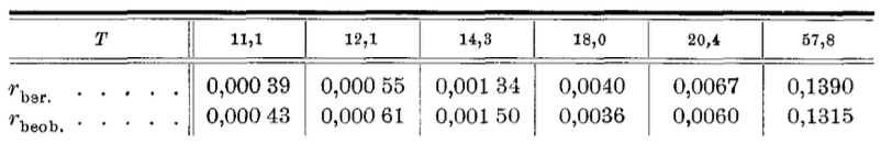
If one uses the $T^4$ law demanded by Grüneisen instead of (11a), one obtains deviations of the same order of magnitude from the measurement results, so that one cannot decide in favor of one or the other. From our formulas (9a and 9b), you also get a quantitative statement about the ratio of the resistance at high and low temperatures. If you put it for $T\gg\Theta$,
$$r=\lambda_2 T,\label{11b}\tag{11b}$$
according to (9a and 9b), it must apply:
$$\frac{\lambda_1}{\lambda_2}=\frac{2\Theta}{\Theta^5/250}=\frac{500}{\Theta^4}.$$
If one calculates the characteristic temperature $\Theta$ from this experimentally known ratio, one obtains, e.g. for gold $\Theta=175$ instead of $\Theta=190$. The deviation of about 10% is well within the error limit caused by our simplifying.